Linear Mappings
이번 장에서는 구조를 유지하는 vector space의 mappings에 대해 살펴보도록 하겠습니다. 이를 통해서 좌표(coordinate)의 개념을 정의할 수 있습니다. 2장의 시작 부분에서 벡터는 벡터 끼리 더할 수 있고 스칼라로 곱할 수 있는 객체(object)라고 정의했으며, 이 연산들의 결과는 다른 벡터가 된다고 언급했습니다.
여기서 mapping을 적용할 때 우리는 이 속성이 유지되는 것을 원합니다. 두 개의 실수 vector space $V, W$ 가 있다고 가정해봅시다. 이때, 아래의 조건이 성립하면
\[\begin{align*} \Phi(\boldsymbol{x} + \boldsymbol{y}) &= \Phi(\boldsymbol{x}) + \Phi(\boldsymbol{y}) \tag{2.85} \\ \Phi(\lambda\boldsymbol{x}) &= \lambda\Phi(\boldsymbol{x}) \tag{2.86} \end{align*}\]mapping $\Phi : V \rightarrow W$ 는 vector space의 구조를 유지합니다 (all $\boldsymbol{x}, \boldsymbol{y} \in V$ and $\lambda \in \mathbb{R}$ 에 대해). 이를 다음과 같이 요약할 수 있습니다.
Definition 2.15 (LInear Mapping). 모든 vector space $V, W$ 에 대해, mapping $\Phi : V \rightarrow W$ 가 아래의 조건을 만족하면,
\[\forall\boldsymbol{x}, \boldsymbol{y} \in V, \quad \forall \lambda, \psi \in \mathbb{R} : \Phi(\lambda\boldsymbol{x} + \psi\boldsymbol{y}) = \lambda\Phi(\boldsymbol{x}) + \psi\Phi(\boldsymbol{y}) \tag{2.87}\]mapping $\Phi$ 를 linear mapping (or vector space homomorphism/linear transformation) 이라고 합니다.
linear mapping은 행렬로 표현할 수 있습니다(2.7.1장). 그리고 vector space를 행렬의 열로 모을 수 있으므로 행렬로 작업할 때는 행렬이 표현하는 것이 무엇인지 알고 있어야 합니다 (ex, linear mapping or a collection of vectors). 4장에서 linear mapping에 대해 조금 더 자세히 살펴봅니다.
이번 장에서는 먼저 special mappings이라는 것을 간략하게 살펴보도록 넘어가도록 하겠습니다.
Defitnition 2.16 (Injective, Surjective, Bijective). 임의의 집합 $\mathcal{V}, \mathcal{W}$ 에 대해 mapping $\Phi : \mathcal{V} \rightarrow \mathcal{W}$ 가 있다고 가정해봅시다. 이때, mapping $\Phi$ 는
- Injective if $\forall\boldsymbol{x}, \boldsymbol{y} \in \mathcal{V} : \Phi(\boldsymbol{x}) = \Phi(\boldsymbol{y}) \implies \boldsymbol{x} = \boldsymbol{y}$ .
- Surjective if $\Phi(\mathcal{V}) = \mathcal{W}$ .
- Bijective if it is injective and surjective.
만약 $\Phi$ 가 surjective라면, $\Phi$ 를 사용하여 $V$ 를 통해 $W$ 의 모든 요소를 얻을 수 있습니다. bijective인 $\Phi$ 는 “undone”할 수 있는데, 이는 mapping $\Psi : \mathcal{W} \rightarrow \mathcal{V}$ 가 존재하고 $\Psi \circ \Phi(\boldsymbol{x}) = \boldsymbol{x}$ 라는 것을 의미합니다. 따라서 mapping $\Psi$ 는 $\Phi$ 의 역이면 일반적으로 $\Phi^{-1}$ 로 표기합니다.
이러한 정의들을 기반으로 아래는 vector space $V$ 와 $W$ 간 linear mapping의 special cases 입니다.
- Isomorphism : $\Phi : V \rightarrow W$ linear and bijective
- Endomorphism : $\Phi : V \rightarrow V$ linear
- Automorphism : $\Phi: V \rightarrow V$ linear and bijective
- $\text{id}_V : V \rightarrow V, \boldsymbol{x} \mapsto \boldsymbol{x}$ (identity mapping or identity automorphism in $V$ )
Example 2.19 (Homomorphism)
mapping $\Phi : \mathbb{R}^2 \rightarrow \mathbb{C}, \Phi(\boldsymbol{x}) = x_1 + ix_2$ 는 homomorphism 입니다:
\[\begin{align*} \Phi\left(\begin{bmatrix} x_1 \\ x_2 \end{bmatrix} + \begin{bmatrix} y_1 \\ y_2 \end{bmatrix} \right) &= (x_1 + y_1) + i(x_2 + y_2) = x_1 + ix_2 + y_1 + iy_2 \\ &= \Phi\left( \begin{bmatrix} x_1 \\ x_2 \end{bmatrix} \right) + \Phi\left( \begin{bmatrix} y_1 \\ y_2 \end{bmatrix} \right) \\ \Phi\left( \lambda\begin{bmatrix} x_1 \\ x_2 \end{bmatrix} \right) &= \lambda x_1 + \lambda i x_2 = \lambda(x_1 + ix_2) = \lambda\Phi\left( \begin{bmatrix} x_1 \\ x_2 \end{bmatrix} \right) \end{align*} \tag{2.88}\]이는 복소수가 $\mathbb{R}^2$ 에서의 튜플로 표현될 수 있다는 것을 보여줍니다.
교재에서는 bijective linear mapping 도 언급하는데, $\mathbb{R}^2$ 의 튜플이 복소수 집합으로 mapping이 되고, 그 반대로 복소수에서 실수부, 허수부를 분리하여 $\mathbb{R}^2$ 의 튜플로도 mapping할 수 있기 때문인 것으로 보입니다… !
Theorem 2.17. Finite-dimensional vector spaces인 $V$ 와 $W$ 가 있을 때, 만약 $\text{dim}(V) = \text{dim}(W)$ 라면, $V$ 와 $W$ 는 isomorphic 하다고 합니다.
이는 같은 차원의 두 vector spaces 간의 linear, bijective mapping이 존재한다는 것을 의미합니다. 즉, 손실없이 서로 변환될 수 있기 때문에 같은 차원의 vector spaces들은 서로 같은 종류의 것이라는 것을 의미합니다.
Theorem 2.17은 우리가 $\mathbb{R}^{m \times n}$ (vector space of $m \times n$ -matrices) 와 $\mathbb{R}^{mn}$ (vector space of vectors of length $mn$ )을 같은 것으로 취급할 수 있도록 해줍니다. 이는 두 vector space가 동일한 차원이고, 그들간의 linear/bijective mapping이 존재하기 때문입니다.
Matrix Representation of Linear Mappings
Theorem 2.17에 의해서 어느 n-차원의 vector space는 $\mathbb{R}^n$ 에 대해 isomorphic 합니다. n 차원의 vector space $V$ 의 basis $\lbrace \boldsymbol{b}_1, \dotsc, \boldsymbol{b}_n \rbrace$ 가 있을 때, basis 벡터의 순서는 아주 중요합니다. 이를 정렬하여 n-튜플로 나타낸 것을 ordered basis of $V$ 라고 하며 다음과 같이 작성합니다.
\[B = (\boldsymbol{b}_1, \cdots, \boldsymbol{b}_n) \tag{2.89}\]Definition 2.18 (Coordinate). vector space $V$ 와 $V$ 의 ordered basis $B = (\boldsymbol{b}_1, \dotsc, \boldsymbol{b}_n)$ 가 있을 때, any $\boldsymbol{x} \in V$ 는 $B$ 에 대한 유일한 linear combination 으로 다음과 같이 표현할 수 있습니다.
\[\boldsymbol{x} = \alpha_1\boldsymbol{b}_1 + \cdots + \alpha_n\boldsymbol{b}_n \tag{2.90}\]이때, $\alpha_1, \dotsc, \alpha_n$ 는 $B$ 에 대한 $\boldsymbol{x}$ 의 coordinate (좌표)이고, 다음의 벡터는
\[\boldsymbol{\alpha} = \begin{bmatrix} \alpha_1 \\ \vdots \\ \alpha_n \end{bmatrix} \in \mathbb{R}^n \tag{2.91}\]ordered basis $B$ 에 대한 $\boldsymbol{x}$ 의 coordinate vector 또는 coordinate representation 입니다.
basis는 좌표계를 효과적으로 정의합니다. canonical basis vectors $\boldsymbol{e}_1, \boldsymbol{e}_2$ 로 span되는 2차원의 데카르트 좌표계(Cartesian coordinate system, link)에 익숙하실지 모르겠습니다. 이 좌표계에서 벡터 $\boldsymbol{x} \in \mathbb{R}^2$ 는 $\boldsymbol{e}_1, \boldsymbol{e}_2$ 의 선형 조합으로 표현됩니다. 그러나 $\mathbb{R}^2$ 의 어떠한 basis 도 유효한 좌표계를 정의하기 때문에, 동일한 벡터 $\boldsymbol{x}$ 는 $(\boldsymbol{b}_1, \boldsymbol{b}_2)$ 에서 다른 좌표계를 가질 수도 있습니다. 아래의 Figure 2.의 왼쪽 그래프는 standard basis $(\boldsymbol{e}_1, \boldsymbol{e}_2)$ 에 대한 $\boldsymbol{x} = \lbrack2, 2,\rbrack^\top$ 를 보여줍니다.
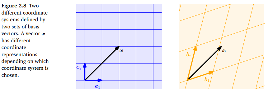
그러나, 오른쪽 그래프는 basis $(\boldsymbol{b}_1, \boldsymbol{b}_2)$ 에 대해 동일한 벡터 $\boldsymbol{x}$ 가 $\lbrack 1.09, 0.72 \rbrack^\top$ 이라는 것을 보여줍니다. 즉, $\boldsymbol{x} = 1.09\boldsymbol{b}_1 + 0.72\boldsymbol{b}_2$ 입니다.
Example 2.20
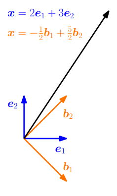
$\mathbb{R}^2$ 의 standard basis $(\boldsymbol{e}_1, \boldsymbol{e}_2)$ 에 대한 geometric vector $\boldsymbol{x} \in \mathbb{R}^2$ 의 좌표가 $\lbrack 2, 3 \rbrack^\top$ 인 경우를 살펴봅시다. 이는 $\boldsymbol{x} = 2\boldsymbol{e}_1 + 3\boldsymbol{e}_2$ 로 표현할 수 있습니다. 그러나 우리는 꼭 이 벡터를 표현할 때 standard basis를 선택할 필요가 없습니다. 만약 basis vectors를 $\boldsymbol{b}_1 = \lbrack 1, -1 \rbrack^\top, \boldsymbol{b}_2 = \lbrack 1, 1 \rbrack^\top$ 으로 선택한다면, 동일한 벡터 $\boldsymbol{x}$ 에 대해서 $\frac{1}{2} \lbrack -1, 5 \rbrack^\top$ 이라는 좌표를 얻을 수 있습니다.
이제 행렬과 유한한 차원의 vector spaces의 linear mapping을 명시적으로 연결시켜보도록 하겠습니다.
Definition 2.19 (Transformation Matrix). Vector spaces $V, W$ 와 이에 대응되는 (ordered) bases $B = (\boldsymbol{b}_1, \dotsc, \boldsymbol{b}_n)$ 과 $C = (\boldsymbol{c}_1, \dotsc, \boldsymbol{c}_m)$ 가 있다고 합시다. 그리고 linear mapping $\Phi : V \rightarrow W$ 가 있을 때,
\[\Phi(\boldsymbol{b}_j) = \alpha_{1j}\boldsymbol{c}_1, + \cdots + \alpha_{mj}\boldsymbol{c}_m = \sum_{i=1}^m \alpha_{ij}\boldsymbol{c}_i \tag{2.92}\]
$j \in \lbrace1, \dotsc, n\rbrace$ 에 대해는 $C$ 에 대한 $\Phi(\boldsymbol{b}_j)$ 의 유일한 표현입니다. 그리고, $m \times n$ -matrix $\boldsymbol{A}_\Phi$ 를 transformation matrix of $\Phi$ 라고 하며, 아래로 표현되는 요소들을 가집니다.
\[A_\Phi(i, j) = \alpha_{ij} \tag{2.93}\]
$\Phi(\boldsymbol{b}_j)$ 의 좌표는 $\boldsymbol{A}_\Phi$ 의 j-th column 입니다.
유한한 차원의 vector spaces $V, W$ 와 이들의 ordered basis $B, C$ , 그리고 transformation matrix $\boldsymbol{A}_\Phi$ 로 주어지는 linear mapping $\Phi : V \rightarrow W$ 가 있다고 합시다. 만약 $\hat{\boldsymbol{x}}$ 가 $B$ 에 대한 $\boldsymbol{x} \in V$ 이고, $\hat{\boldsymbol{y}}$ 가 $C$ 에 대한 $\boldsymbol{y} = \Phi(\boldsymbol{x}) \in W$ 이라면,
\[\hat{\boldsymbol{y}} = \boldsymbol{A}_\Phi\hat{\boldsymbol{x}} \tag{2.94}\]입니다.
이는 transformation matrix를 $V$ 의 ordered basis에 대한 좌표를 $W$ 의 ordered basis에 대한 좌표로 mapping하는데 사용할 수 있다는 것을 의미합니다.
Example 2.21 (Transformation Matrix)
\[\begin{align*} \Phi(\boldsymbol{b}_1) &= \boldsymbol{c}_1 - \boldsymbol{c}_2 + 3\boldsymbol{c}_3 - \boldsymbol{c}_4 \\ \Phi(\boldsymbol{b}_2) &= 2\boldsymbol{c}_1 + \boldsymbol{c}_2 + 7\boldsymbol{c}_3 + 2\boldsymbol{c}_4 \\ \Phi(\boldsymbol{b}_3) &= 3\boldsymbol{c}_2 + \boldsymbol{c}_3 + 4\boldsymbol{c}_4 \end{align*} \tag{2.95}\]
Homomorphism한 mapping $\Phi : V \rightarrow W$ 와 $V$ 의 ordered basis $B = (\boldsymbol{b}_1, \dotsc, \boldsymbol{b}_3)$, $W$ 의 ordered basis $C = (\boldsymbol{c}_1, \dotsc, \boldsymbol{c}_4)$ 가 있다고 합시다.일 때, $B$ 와 $C$ 에 대한 transformation matrix $\boldsymbol{A}_\Phi$ 는 $\Phi(\boldsymbol{b}_k) = \sum_{i=1}^4 \alpha_{ik}\boldsymbol{c}_i, \text{ } k = 1, \dotsc, 3$ 을 만족하며, 다음과 같이 주어집니다.
\[\boldsymbol{A}_\Phi = \lbrack \boldsymbol{\alpha}_1, \boldsymbol{\alpha}_2, \boldsymbol{\alpha}_3 \rbrack = \begin{bmatrix} 1 & 2 & 0 \\ -1 & 1 & 3 \\ 3 & 7 & 1 \\ -1 & 2 & 4 \end{bmatrix} \tag{2.96}\]이때, $\boldsymbol{\alpha}_j \text{ } (j = 1,2,3)$ 은 $C$ 에 대한 $\Phi(\boldsymbol{b}_j)$ 의 좌표 벡터입니다.
Example 2.22 (Linear Transformations of Vectors)
다음의 transformation matrices 를 가지고 $\mathbb{R}^2$ 의 벡터 집합의 linear transformation 에 대해 살펴보도록 하겠습니다.
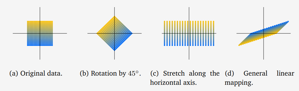
\[\boldsymbol{A}_1 = \begin{bmatrix} \cos(\frac{\pi}{4}) & -\sin(\frac{\pi}{4}) \\ \sin(\frac{\pi}{4}) & \cos(\frac{\pi}{4}) \end{bmatrix}, \boldsymbol{A}_2 = \begin{bmatrix} 2 & 0 \\ 0 & 1 \end{bmatrix}, \boldsymbol{A}_3 = \frac{1}{2}\begin{bmatrix} 3 & -1 \\ 1 & -1 \end{bmatrix} \tag{2.97}\]아래 그림은 위의 3개의 transformation을 그래프로 표현한 것 입니다.
(a)는 $\mathbb{R}^2$ 에서 400개의 벡터를 표현하고 있으며, 각각은 $(x_1, x_2)$ 좌표에 대응합니다.
식 (2.97)의 $\boldsymbol{A}_1$ 행렬을 사용하여 (a)의 벡터들을 선형 변환하면 (b)에서 보여주는 것과 같이 회전한 사각형을 얻을 수 있습니다. $\boldsymbol{A}_2$ 를 사용하면 (c)와 같이 $x_1$ 축으로 늘어난 사각형을 얻을 수 있습니다. (d)의 경우에는 $\boldsymbol{A}_3$ 을 사용하여 linear transformation한 결과이며 reflection/rotation/stretch 이 모두 적용되었습니다.
Basis Change
이번에는 $V$ 와 $W$ 의 basis들을 변경했을 때, linear mapping $\Phi : V \rightarrow W$ 의 transformation matrix들이 어떻게 되는지 자세히 살펴보도록 하겠습니다.
$V$ 의 두 ordered basis가 다음과 주어지고,
\[B = (\boldsymbol{b}_1, \dotsc, \boldsymbol{b}_n), \quad \tilde{B} = (\tilde{\boldsymbol{b}}_1, \dotsc, \tilde{\boldsymbol{b}}_n) \tag{2.98}\]$W$ 의 두 ordered basis는 다음과 같이 주어졌다고 합시다.
\[C = (\boldsymbol{c}_1, \dotsc, \boldsymbol{c}_m), \quad \tilde{C} = (\tilde{\boldsymbol{c}}_1, \dotsc, \tilde{\boldsymbol{c}}_m) \tag{2.99}\]또한, $B$ 와 $C$ 에 대한 linear mapping $\Phi : V \rightarrow W$ 의 transformation matrix를 $\boldsymbol{A}_\Phi \in \mathbb{R}^{m \times n}$ 이라고 하고, $\tilde{B}$ 와 $\tilde{C}$ 에 대한 linear mapping의 transformation matrix를 $\tilde{\boldsymbol{A}}_\Phi \in \mathbb{R}^{m \times n}$ 이라고 합시다.
이때, 만약 basis를 $B, C$ 에서 $\tilde{B}, \tilde{C}$ 로 변경하면 어떻게 $\boldsymbol{A}_\Phi$ 에서 $\tilde{\boldsymbol{A}}_\Phi$ 로 변환할 수 있는지에 대해 살펴보도록 하겠습니다.
Example 2.23 (Basis Change)
\[\boldsymbol{A} = \begin{bmatrix} 2 & 1 \\ 1 & 2 \end{bmatrix} \tag{2.100}\]
$\mathbb{R}^2$ 의 canonical basis 에 대해 transformation matrix가 다음과 같이 주어졌다고 가정합니다.만약, 새로운 basis를 다음과 같이 정의한다면,
\[B = (\begin{bmatrix} 1 \\ 1 \end{bmatrix}, \begin{bmatrix} 1 \\ -1 \end{bmatrix}) \tag{2.101}\]$B$ 에 대해서 다음과 같은 diagonal transformation matrix
\[\tilde{\boldsymbol{A}} = \begin{bmatrix} 3 & 0 \\ 0 & 1 \end{bmatrix} \tag{2.102}\]을 얻을 수 있습니다. 새롭게 얻은 transformation matrix를 사용하면 기존보다 연산이 더 쉬워집니다.
\[\begin{align*} \boldsymbol{B}^{-1}\boldsymbol{AB} &= \begin{bmatrix}1&1\\1&-1\end{bmatrix}^{-1}\begin{bmatrix}2&1\\1&2\end{bmatrix}\begin{bmatrix}1&1\\1&-1\end{bmatrix} \\ &= \frac{1}{2}\begin{bmatrix}1&1\\1&-1\end{bmatrix}\begin{bmatrix}2&1\\1&2\end{bmatrix}\begin{bmatrix}1&1\\1&-1\end{bmatrix} = \begin{bmatrix}3&0\\0&1\end{bmatrix} \end{align*}\]
참고로, $\hat{\boldsymbol{A}}$ 는 $\boldsymbol{B}^{-1}\boldsymbol{AB}$ 를 계산하면 얻을 수 있습니다. 여기서 $\boldsymbol{B}$ 는 새로운 basis의 column으로 구성된 행렬입니다. 따라서, 다음과 같이 계산합니다.3Blue1Brown 이라는 유튜브 채널의 영상(link)에서 이를 시각적으로 이해가 쉽도록 설명해줍니다. 필요하시다면 참조하시길 바랍니다 !
Theorem 2.20 (Basis Change). Linear mapping $\Phi : V \rightarrow W$ 에 대해, $V$ 의 ordered basis들이 다음과 같고,
\[B = (\boldsymbol{b}_1, \dotsc, \boldsymbol{b}_n), \quad \tilde{B} = (\tilde{\boldsymbol{b}}_1, \dotsc, \tilde{\boldsymbol{b}}_n) \tag{2.103}\]$W$ 의 rodered basis들은 다음과 같을 때,
\[C = (\boldsymbol{c}_1, \dotsc, \boldsymbol{c}_m), \quad \tilde{C} = (\tilde{\boldsymbol{c}}_1, \dotsc, \tilde{\boldsymbol{c}}_m) \tag{2.104}\]$B, C$ 에 대한 transformation matrix $\boldsymbol{A}_\Phi$ 와 $\tilde{B}, \tilde{C}$ 에 대한 transformation matrix $\tilde{\boldsymbol{A}}_\Phi$ 의 관계는 다음의 식으로 주어집니다 (다음의 식을 아래에서 그림으로 표현한 것이 있는데, 함께 보는 것을 추천드립니다).
\[\tilde{\boldsymbol{A}}_\Phi = \boldsymbol{T}^{-1}\boldsymbol{A}_\Phi \boldsymbol{S} \tag{2.105}\]이때, $\boldsymbol{S} \in \mathbb{R}^{n \times n}$ 은 $\tilde{B}$ 에 대한 좌표를 $B$ 에 대한 좌표로 변환하는 $\text{id}_V$ 의 transformation matrix 이며, $\boldsymbol{T} \in \mathbb{R}^{m \times m}$ 은 $\tilde{C}$ 에 대한 좌표를 $C$ 에 대한 좌표로 변환하는 $\text{id}_W$ 의 transformation matrix 입니다.
Theorem 2.20에 대한 증명은 생략하도록 하겠습니다 (교재 참조).
이를 그림으로 표현하면 다음과 같습니다. 각각의 mapping에서의 transformation matrix를 $\boldsymbol{A}_\Phi, \boldsymbol{S}, \tilde{\boldsymbol{A}}_\Phi, \boldsymbol{T}$ 로 나타내고 있습니다.
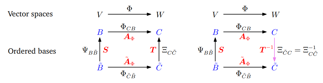
위 그림을 통해, 이전의 basis $B, C$ 에서 새로운 basis $\tilde{B}, \tilde{C}$ 로 변환했을 때, 변환된 linear mapping $\Phi_{\tilde{C}\tilde{B}}$ 을 기존의 basis로 표현하면 다음과 같이 표현할 수 있습니다.
\[\Phi_{\tilde{C}\tilde{B}} = \Theta_{\tilde{C}C}\circ\Phi_{CB}\circ\Psi_{B\tilde{B}} = \Theta_{C\tilde{C}}^{-1}\circ\Phi_{CB}\circ\Psi_{B\tilde{B}} \tag{2.114}\]Definition 2.21 (Equivalence). 만약 $\tilde{\boldsymbol{A}} = \boldsymbol{T}^{-1}\boldsymbol{AS}$ 인 regular matrix $\boldsymbol{S} \in \mathbb{R}^{n \times n}$ 과 $\boldsymbol{T}\in\mathbb{R}^{m \times m}$ 이 존재한다면, 두 행렬 $\boldsymbol{A}, \tilde{\boldsymbol{A}} \in \mathbb{R}^{m \times n}$ 은 equivalent 하다고 합니다.
Definition 2.22 (Similarity). 만약 $\tilde{\boldsymbol{A}} = \boldsymbol{S}^{-1}\boldsymbol{AS}$ 인 regular matrix $\boldsymbol{S} \in \mathbb{R}^{n \times n}$ 이 존재한다면, 두 행렬 $\boldsymbol{A}, \tilde{\boldsymbol{A}} \in \mathbb{R}^{m \times n}$ 은 similar 하다고 합니다.
Theorem 2.20에서 각 basis 변환을 다음과 같이 표현할 때,
\[\begin{align*} \boldsymbol{A}_\Phi : B \rightarrow C \\ \tilde{\boldsymbol{A}}_\Phi : \tilde{B} \rightarrow \tilde{C} \\ \boldsymbol{S} : \tilde{B} \rightarrow B \\ \boldsymbol{T} : \tilde{C} \rightarrow C \end{align*}\]식 (2.105)는 다음과 같습니다.
\[\tilde{B} \rightarrow \tilde{C} = \tilde{\color{Blue}B} \color{Blue}\rightarrow \color{Blue}B \color{Red}\rightarrow \color{Red}C \rightarrow \tilde{C} \tag{2.115}\] \[\tilde{\boldsymbol{A}}_\Phi = \boldsymbol{T}^{-1} \boldsymbol{\color{Red}A}_{\color{Red}\Phi} \boldsymbol{\color{Blue}S} \tag{2.116}\]식 (2.116)의 순서에 주의해야 합니다 ($\boldsymbol{x} \mapsto \boldsymbol{Sx} \mapsto \boldsymbol{A}_\Phi(\boldsymbol{Sx}) \mapsto \boldsymbol{T}^{-1}(\boldsymbol{A}_\Phi(\boldsymbol{Sx})) = \tilde{\boldsymbol{A}}_\Phi\boldsymbol{x}$ ).
Example 2.24 (Basis Change)
\[B = (\begin{bmatrix}1 \\ 0 \\ 0\end{bmatrix}, \begin{bmatrix}0\\1\\0\end{bmatrix}, \begin{bmatrix}0\\0\\1\end{bmatrix}), \quad C = (\begin{bmatrix}1\\0\\0\\0\end{bmatrix},\begin{bmatrix}0\\1\\0\\0\end{bmatrix},\begin{bmatrix}0\\0\\1\\0\end{bmatrix},\begin{bmatrix}0\\0\\0\\1\end{bmatrix}) \tag{2.118}\]
표준 기저(standard basis)에 대해, Linear mapping $\Phi : \mathbb{R}^3 \rightarrow \mathbb{R}^4$ 의 transformation matrix가 다음과 같다고 합시다.
\[\boldsymbol{A}_\Phi = \begin{bmatrix} 1 & 2 & 0 \\ -1 & 1 & 3 \\ 3 & 7 & 1 \\ -1 & 2 & 4 \end{bmatrix} \tag{2.117}\]이때, 새로운 basis
\[\tilde{B} = (\begin{bmatrix}1 \\ 1 \\ 0\end{bmatrix}, \begin{bmatrix}0\\1\\1\end{bmatrix}, \begin{bmatrix}1\\0\\1\end{bmatrix}), \quad \tilde{C} = (\begin{bmatrix}1\\1\\0\\0\end{bmatrix},\begin{bmatrix}1\\0\\1\\0\end{bmatrix},\begin{bmatrix}0\\1\\1\\0\end{bmatrix},\begin{bmatrix}1\\0\\0\\1\end{bmatrix}) \tag{2.119}\]에 대한 mapping $\Phi$ 의 transformation matrix $\tilde{\boldsymbol{A}}_\Phi$ 를 찾고자 합니다.
\[\boldsymbol{S} = \begin{bmatrix} 1 & 0 & 1 \\ 1 & 1 & 0 \\ 0 & 1 & 1 \end{bmatrix}, \quad \boldsymbol{T} = \begin{bmatrix} 1 & 1 & 0 & 1 \\ 1 & 0 & 1 & 0 \\ 0 & 1 & 1 & 0 \\ 0 & 0 & 0 & 1 \end{bmatrix} \tag{2.120}\]
Standard basis이기 때문에 $\tilde{B} \rightarrow B, \tilde{C} \rightarrow C$ 의 transformation matrix $\boldsymbol{S}, \boldsymbol{T}$ 는 쉽게 구할 수 있습니다.그리고 (2.116) 공식을 활용하면, $\tilde{\boldsymbol{A}}_\Phi$ 를 구할 수 있습니다.
\[\begin{align*} \tilde{\boldsymbol{A}}_\Phi = \boldsymbol{T}^{-1}\boldsymbol{A}_\Phi\boldsymbol{S} &= \frac{1}{2}\begin{bmatrix} 1&1&-1&-1\\1&-1&1&-1\\-1&1&1&1\\0&0&0&2 \end{bmatrix}\begin{bmatrix}1&2&0\\-1&1&3\\3&7&1\\-1&2&4\end{bmatrix}\begin{bmatrix}1&0&1\\1&1&0\\0&1&1\end{bmatrix} \\ &= \begin{bmatrix}-4&-4&-2\\6&0&0\\4&8&4\\1&6&3\end{bmatrix} \end{align*} \tag{2.121}\]
Image and Kernel
교재를 보기 전에 3Blue1Brown 유튜브 영상(link)를 먼저 보시면 더 쉽게 이해할 수 있습니다 !
Linear mapping에서의 iamge와 kernel은 중요한 속성들을 가진 vector space 입니다.
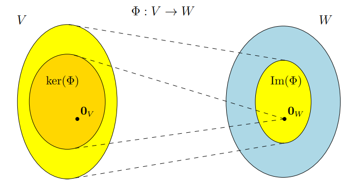
Definition 2.23 (Image and Kernel)
\[\text{ker}(\Phi) := \Phi^{-1}(\boldsymbol{0}_W) = \lbrace \boldsymbol{v} \in V : \Phi(\boldsymbol{v}) = \boldsymbol{0}_W \rbrace \tag{2.122}\]
$\Phi : V \rightarrow W$ 에 대해 kernel/null space 는 다음과 같이 정의되고,image/range 는 다음으로 정의됩니다.
\[\text{Im}(\Phi) := \Phi(V) = \lbrace \boldsymbol{w} \in W | \exists\boldsymbol{v} \in V : \Phi(\boldsymbol{v}) = \boldsymbol{w} \rbrace \tag{2.123}\]
그리고, $V$ 와 $W$ 를 각각 $\Phi$ 의 domain 과 codomain 이라고 부릅니다.
직관적으로 이야기하면, kernel은 $\Phi$ 가 항등원(neutral element) $\boldsymbol{0}_W \in W$ 으로 매핑되는 $\boldsymbol{v} \in V$ 의 벡터 집합이고, image는 $V$ 의 어떠한 벡터가 $\Phi$ 로부터 벡터 $\boldsymbol{w} \in W$ 로 매핑되는 벡터 집합입니다. 그림으로 표현하면 다음과 같습니다.
Example 2.25 (Image and Kernel of a Linear Mapping)
\[\begin{align*} \Phi : \mathbb{R}^4 \rightarrow \mathbb{R}^2, \begin{bmatrix}x_1\\x_2\\x_3\\x_4\end{bmatrix}&\mapsto\begin{bmatrix}1&2&-1&0\\1&0&0&1\end{bmatrix}\begin{bmatrix}x_1\\x_2\\x_3\\x_4\end{bmatrix} = \begin{bmatrix}x_1 + 2x_2 -x_3\\x_1+x_4\end{bmatrix} \\ &= x_1\begin{bmatrix}1\\1\end{bmatrix} + x_2\begin{bmatrix}2\\0\end{bmatrix} + x_3\begin{bmatrix}-1\\0\end{bmatrix} + x_4\begin{bmatrix}0\\1\end{bmatrix} \end{align*} \tag{2.125}\]
아래의 mapping은 linear 합니다.$\text{Im}(\Phi)$ 를 결정하기 위해서 transformation matrix의 열들의 span을 취하면, 다음을 얻을 수 있습니다.
\[\text{Im}(\Phi) = \text{span}\lbrack \begin{bmatrix}1\\1\end{bmatrix}, \begin{bmatrix}2\\0\end{bmatrix}, \begin{bmatrix}-1\\0\end{bmatrix}, \begin{bmatrix}0\\1\end{bmatrix} \rbrack \tag{2.126}\]$\Phi$ 의 kernel (null space)를 계산하기 위해서, $\boldsymbol{Ax} =\boldsymbol{0}$ 의 해를 구해야 합니다. 이를 풀기 위해 가우스 소거법을 사용하여 $\boldsymbol{A}$ 를 reduced row-echelon form으로 변환하면 다음과 같습니다.
\[\begin{bmatrix}1&2&-1&0\\1&0&0&1\end{bmatrix} \rightsquigarrow \cdots \rightsquigarrow \begin{bmatrix}1&0&0&1\\0&1&-\frac{1}{2}&-\frac{1}{2}\end{bmatrix} \tag{2.127}\]그리고, Minus-1 Trick을 사용하여 다음과 같이 kernel의 basis를 구합니다 (2.3.3장 참고).
\[\begin{bmatrix}1&0&0&1\\0&1&-\frac{1}{2}&-\frac{1}{2}\end{bmatrix} \rightsquigarrow \begin{bmatrix}1&0&0&1\\0&1&-\frac{1}{2}&-\frac{1}{2}\\0&0&-1&0\\0&0&0&-1\end{bmatrix}\]위 결과의 3열과 4열을 통해 결정된 kernel은 다음과 같습니다.
\[\text{ker}(\Phi) = \text{span}\lbrack \begin{bmatrix}0\\\frac{1}{2}\\1\\0 \end{bmatrix} , \begin{bmatrix}-1\\\frac{1}{2}\\0\\1\end{bmatrix} \rbrack \tag{2.128}\]또는, 식 (2.127)의 결과 행렬에서 3,4열을 1,2열의 linear combination으로 표현하여 구할 수 있습니다. 3열 $\boldsymbol{a}_3$ 은 2열에서 $-\frac{1}{2}$ 배 한 것이므로 $\boldsymbol{0} = \boldsymbol{a}_3 + \frac{1}{2}\boldsymbol{a}_2$ 입니다. 동일한 방식으로 $\boldsymbol{a}_4 = \boldsymbol{a}_1 - \frac{1}{2}\boldsymbol{a}_2$ 이며 $\boldsymbol{0} = \boldsymbol{a}_1 - \frac{1}{2}\boldsymbol{a}_2 -\boldsymbol{a}_4$ 입니다. 종합하면, (2.128)과 같은 결과를 얻을 수 있습니다.
Definition 2.24 (Rank-Nullity Theorem). Vector spaces $V, W$ 와 linear mapping $\Phi : V \rightarrow W$ 가 있을 때, 다음이 성립합니다.
\[\text{dim}(\text{ker}(\Phi)) + \text{dim}(\text{Im}(\Phi)) = \text{dim}(V) \tag{2.129}\]
Rank-nullity theorem은 fundamental theorem of linear mappings 라고도 칭하며, 다음과 같은 성질들을 가지고 있습니다.
- $\text{dim}(\text{Im}(\Phi)) < \text{dim}(V)$ 라면, $\text{ker}(\Phi)$ 는 non-trivial 입니다. 즉, kernel 은 $\boldsymbol{0}_V$ 이외를 포함하며 $\text{dim}(\text{ker}(\Phi)) \geq 1$ 입니다.
- $\boldsymbol{A}_\Phi$ 가 ordered basis에 대한 $\Phi$ 의 transformation matrix 이고 $\text{dim}(\text{Im}(\Phi)) < \text{dim}(V)$ 라면, 연립선형방정식 $\boldsymbol{A}_\Phi\boldsymbol{x} = \boldsymbol{0}$ 은 무한히 많은 해를 가집니다.
- $\text{dim}(V) = \text{dim}(W)$ 라면, $\Phi$ 는 injective, surjective, bijective 합니다.