Vector Spaces
이번 절에서는 벡터 공간(vector spaces), 즉, 벡터가 존재하는 구조화된 공간에 대해서 살펴보도록 하겠습니다.
2장을 시작할 때, 벡터를 동일한 벡터로 더하거나 스칼라를 곱할 수 있는 객체로 비공식적으로 정의했습니다. 이번에는 이를 공식화할텐데, 먼저 group(군)이라는 개념을 소개하도록 하겠습니다.
Groups
Groups(군)은 컴퓨터 공학에서 중요한 역할을 합니다. 집합에 대한 연산을 제공하는 기본적인 프레임워크를 제공하는 것 이외에도 cryptography, coding theory, graphics에서도 많이 사용됩니다.
Definition 2.7 (Group). 집합 $\mathcal{G}$ 과 연산 $\otimes : \mathcal{G} \times \mathcal{G} \rightarrow \mathcal{G}$ 가 $\mathcal{G}$ 에 대해 정의되어 있을 때, 아래의 조건을 만족하는 $G := (\mathcal{G}, \otimes)$ 를 그룹이라고 부른다.
- Closure of $\mathcal{G}$ on $\otimes : \forall x,y \in \mathcal{G}: x \otimes y \in \mathcal{G}$
- Associativity: $\forall x, y, z \in \mathcal{G}: (x \otimes y) \otimes z = x \otimes (y \otimes z)$ (결합법칙)
- Neutral element: $\exists e \in \mathcal{G}, \forall x \in \mathcal{G} : x \otimes e = x \text{ and } e \otimes x = x$ (항등원)
- Inverse element: $\forall x \in \mathcal{G}, \exists y \in \mathcal{G} : x \otimes y = e \text{ and } y \otimes x = e$ . (역원) 보통 $x^{-1}$ 을 x의 inverse element(역원)이라고 표기합니다. 여기서 $e$ 는 항등원을 나타냅니다.
위 조건에 추가로 $\forall x, y \in \mathcal{G} : x \otimes y = y \otimes x$ 를 만족한다면, $G = (\mathcal{G}, \otimes)$ 를 Abelian group 이라고 합니다 (commutative, 교환법칙이 성립하는 군).
Example 2.10 (Groups)
다음은 group의 관한 몇 가지 예제들입니다.\[(x_1, \cdots, x_n) + (y_1, \cdots, y_n) = (x_1 + y_1, \cdots, x_n + y_n) \tag{2.61}\]
- $(\mathbb{Z}, +)$ is a group.
- $(\mathbb{N}_0, +)$ is not a group. 항등원(0)은 존재하지만 역원이 존재하지 않음 ($\mathbb{N}_0 := \mathbb{N} \cup \lbrace 0 \rbrace$).
- $(\mathbb{Z}, \cdot)$ is not a group. 항등원(1)은 존재하지만 $\pm$ 1이 아닌 모든 z에 대해 역원이 존재하지 않음.
- $(\mathbb{R}, \cdot)$ is not a group. 0에 대한 역원이 존재하지 않음.
- $(\mathbb{R}\backslash\lbrace 0 \rbrace)$ is Abelian.
- $(\mathbb{N}^n, +), (\mathbb{Z}^n, +), n \in \mathbb{N}$ are Abelian if + is defined componentwise, i.e.,
$(x_1, \cdots, x_n)^{-1} := (-x_1, \cdots, -x_n)$ 은 역원이고, 항등원은 $e = (0, \cdots, 0)$ 입니다.
- $(\mathbb{R}^{m\times n}, +)$, the set of $m \times n$ -matrices is Abelian (with componentwise addition as defined in (2.61))
- $(\mathbb{R}^{n\times n}, \cdot)$ , 즉, $n \times n$ 행렬 집합에 대해서 살펴보도록 하겠습니다.
- Matrix multiplication 정의에 의해 Closure과 associativity 성질을 만족합니다.
- 항등행렬(Identity matrix) $\boldsymbol{I}_n$ 은 주어진 조건에서 행렬 곱( $\cdot$ )에 대해 항등원입니다.
- 만약 역행렬이 존재한다면, 즉, $\boldsymbol{A}$ 가 regular 라면, $\boldsymbol{A}^{-1}$ 은 행렬 $\boldsymbol{A} \in \mathbb{R}^{n\times n}$ 의 역행렬입니다. 따라서, $(\mathbb{R}^{n\times n}, \cdot)$ 은 group이며, general limear group 이라고 부릅니다.
Definition 2.8 (General Linear Group). 역행렬이 존재하는 regular matrix $\boldsymbol{A} \in \mathbb{R}^{n \times n}$ 의 집합은 group이며, 이를 general linear group(일반 선형군)이라고 부르며 $GL(n, \mathbb{R})$ 로 표기합니다. 그러나, 행렬 곱은 교환법칙이 성립하지 않기 때문에 Abelian은 아닙니다.
Vector Spaces
위에서 group은 inner operation에 대해서만 고려했는데, 이번에는 벡터와 스칼라의 곱을 의미하는 outer operation인 $\cdot$ 도 포함하는 집합을 살펴봅니다. 여기서 inner operation은 $\mathcal{G}\times\mathcal{G}\rightarrow\mathcal{G}$ 와 같이 오직 $\mathcal{G}$ 의 요소에 대한 연산을 의미합니다. 아래에서는 inner operation $+$ 뿐만 아니라 outer operation $\cdot$ (벡터와 스칼라의 곱) 도 포함하는 집합에 대해 살펴봅니다.
inner opration을 덧셈의 형태, outer operation은 스케일링(scaling)의 형태로 생각할 수 있습니다. inner/outer products(내적/외적)과는 관련이 없습니다.
Definition 2.9 (Vector Spaces). 실수인 벡터 공간 $V = (V, +, \cdot)$ 은 아래 두 연산을 포함하는 집합 $\mathcal{V}$ 입니다.
\[\begin{align*} + &: \mathcal{V} \times \mathcal{V} \rightarrow \mathcal{V} \tag{2.62} \\ \cdot &: \mathbb{R} \times \mathcal{V} \rightarrow \mathcal{V} \tag{2.63} \end{align*}\]
여기서, 벡터 공간은 다음과 같은 특성을 가지고 있습니다.
- $(\mathcal{V}, +)$ is an Abelian group
- Distributivity
- $\forall \lambda \in \mathbb{R}, \boldsymbol{x, y} \in \mathbb{V} : \lambda \cdot (\boldsymbol{x} + \boldsymbol{y}) = \lambda \cdot \boldsymbol{x} + \lambda \cdot \boldsymbol{y}$
- $\forall \lambda, \psi \in \mathbb{R}, \boldsymbol{x} \in \mathbb{V} : (\lambda + \psi)\cdot\boldsymbol{x} = \lambda\cdot\boldsymbol{x} + \psi\cdot\boldsymbol{x}$
- Associativity (outer operation): $\forall\lambda,\psi \in \mathbb{R}, \boldsymbol{x}\in\mathbb{V}: \lambda\cdot(\psi\cdot\boldsymbol{x}) = (\lambda\psi)\cdot\boldsymbol{x}$
- Neutral element with respect to the outer operation: $\forall\boldsymbol{x}\in\mathbb{V} : 1\cdot\boldsymbol{x} = \boldsymbol{x}$
$\boldsymbol{x} \in V$ , 즉, $V$에 속하는 요소들은 벡터(vectors)라고 부릅니다. 벡터 공간에서 항등원은 0-벡터 $\boldsymbol{0} = \lbrack 0, \cdots, 0 \rbrack^\top$ 이고, inner operation은 vector addition이라고 부릅니다. $\lambda \in \mathbb{R}$ 은 스칼라(scalar)라고 부르고 outer operation $\cdot$ 은 multiplication by scalars 입니다. scalar product와는 조금 다른데, 이는 3.2절에서 살펴보도록 하겠습니다.
Vector Subspaces
Vector Subspaces는 직관적으로 이 부분공간 내의 요소들에 대해 벡터 연산을 수행할 때, 원래의 벡터 공간에 포함되는 집합입니다. 따라서, vector subspaces 또한 닫혀(closed) 있습니다. Vector subspaces는 머신러닝에서 중요한 개념이며, 10장에서는 dimensionality reduction에서 이를 어떻게 사용하는지 보여줍니다.
Definition 2.10 (Vector Subspace). $V = (\mathcal{V}, +, \cdot)$ 가 vector space이고, $\mathcal{U} \subseteq \mathcal{V}, \mathcal{U} \neq \emptyset$ 라고 할 때, $U = (\mathcal{U}, +, \cdot)$ 을 $V$ 의 vector subspace(or linear subspace)라고 합니다. 이때, $U$ 는 $\mathcal{U} \times \mathcal{U}$ 와 $\mathbb{R} \times \mathcal{U}$ 로 제한되는 vector space operation $+, \cdot$ 의 vector space 입니다. $V$ 의 subspace $U$ 를 $U \subseteq V$ 로 씁니다.
$\mathcal{U} \subseteq \mathcal{V}$ 이고 $V$ 가 vector spcae라면, $U$는 자연스럽게 $V$ 의 특성을 물려받습니다. 여기에는 abelian group 속성, 분배 법칙, 결합 법칙, 항등원이 포함됩니다. $(\mathcal{U}, +, \cdot)$ 이 $V$ 의 subspace인지 확인하려면 아래의 조건을 만족하는지 확인하면 됩니다.
- $\mathcal{U} \neq \emptyset$ , in particular: $\boldsymbol{0} \in \mathcal{U}$
- Closure of $U$ :
a. With repsect th the outer operation: $\forall\lambda \in \mathbb{R}, \forall\boldsymbol{x} \in \mathcal{U} : \lambda\boldsymbol{x} \in \mathcal{U}$
b. With respect to the inner operation: $\forall\boldsymbol{x, y} \in \mathcal{U} : \boldsymbol{x} + \boldsymbol{y} \in \mathcal{U}$
Example 2.12 (Vector Subspaces) 다음은 vector subspaces의 몇 가지 예제를 보여줍니다.
- 모든 vector space $V$ 에 대해서, 자명한 부분공간(trivial subspaces)는 $V$ 자신과 $\lbrace\boldsymbol{0}\rbrace$ 입니다.
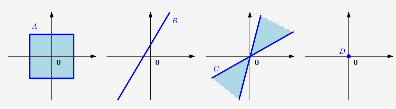
- Figure 2.6의 D만 $\mathbb{R}^2$ 의 subspace 입니다. A와 C는 closure property가 성립하지 않으며, B는 $\boldsymbol{0}$ 을 포함하지 않습니다.
Figure 2.6
- n개의 미지수 $\boldsymbol{x} = \lbrack x_1, \cdots, x_n \rbrack^\top$ 의 homogeneous system of linear equations $\boldsymbol{Ax} = 0$ 의 solution set은 $\mathbb{R}^n$ 의 subspace 입니다.
- inhomogeneous system of linear equations $\boldsymbol{Ax} = \boldsymbol{b}, \boldsymbol{b} \neq \boldsymbol{0}$ 의 solution은 $\mathbb{R}^n$ 의 subspace가 아닙니다.
- 임의의 많은 subspaces의 intersection은 그 자체로 subspace 입니다.